Chapter 10

I Come to Bury Sigma, Not to Praise It

History of Sigma

Although understanding Sigma may not be important for most of us in the 21st century, it would be hard to overestimate its impact on the 19th and first half of the 20th centuries, when it was pretty much the only game in town. Thus if you excavate the foundations of physics, medicine, engineering, economics, statistics and many other fields, you will find Sigma.

It all started with Central Limit Theorem and resulting Normal Distribution, as discussed in Chapter 9. This mathematical result is on the short list of man’s most influential intellectual accomplishments. According to Wikipedia, numerous famous mathematicians were involved, starting with de Moivre in 1734 and Laplace in 1812. But Gauss, who brought additional rigor to the subject in 1809, seems to have ended up winning the trademark, as the bell shaped curve is often called a Gaussian Distribution

Carl Friedrich Gauss on a 10 Mark German Bank Note from the 1990’s: The Boy and His Distribution

The Normal Distribution was really important in the Steam Era for three vital reasons:

Many uncertainties in life involve adding up a bunch of other uncertainties, hence a lot of things are Normally Distributed (see table below).
The powerful mathematics underlying the Normal Distribution allowed many important problems to be solved.
They didn’t have computers

Physics	The velocity of a given air molecule is determined by adding up the results of all the collisions it has had with other air molecules. Hence air molecule velocities are normally distributed.
Biology	The size of a given animal involves averages of the sizes of its ancestors. Hence the size of animals of a given species (along with almost everything else you can measure in biology) tends to be normally distributed.
Finance	In the theory of finance, the prices of securities are often modeled as lognormal (an Uncertain Number whose log is normally distributed).

What Sigma Means

All Normal Distributions look pretty much alike except for two traits.

1. The average or mean, also called mu(µ) measures the distance of the center of the bell from 0.

2. Sigma measures the width of the bell.

Confidence Intervals

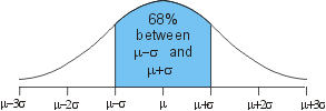
An important fact about the Normal Distribution is that 95% of its occurrences lie within a distance of 2 times Sigma either side of the average. For example, suppose you know that the average length of an adult male giraffe neck is 10 feet, and that Sigma has been computed to be 1 foot. Then, assuming that giraffe neck lengths are Normally Distributed (a pretty good assumption since physical traits tend to be averaged across many ancestors), you can be 95% confident that the next adult male giraffe you see will have a neck between 8 and 12 feet long (2 feet either side of 10).

How is Sigma Computed

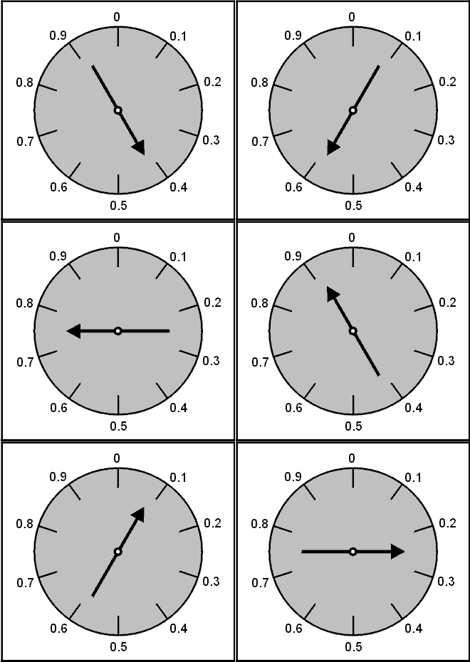
I will try to provide an intuitive explanation of Sigma by showing how it would be determined for the spinner below.

Technically the definition is THE SQUARE ROOT OF THE AVERAGE OF THE SQUARES OF THE DIFFERENCES BETWEEN ALL THE POINTS OF THE DISTRIBUTION AND THE AVERAGE POINT. Could this be why no one understands it?

Finding Sigma for the spinner can be done in a few steps using Calculus, but if you know calculus you probably already know how Sigma is defined, so I will describe a more experiential approach instead that you may not have seen.

First, remember that the average outcome of the spinner was 0.5. We will need this for the calculations ahead. Here goes.

See? That wasn’t so hard. You’ll just have to trust me on the actual number above unless you want to spend a lot of time with a spinner.

Oops sorry, we’re not done. What we found was the Variance or Sigma Squared, not Sigma itself.

Before continuing in our quest for Sigma of the spinner, here is a geometrical interpretation of what we have accomplished so far. Define points in the XY plane with both X and Y values equal to the average, and all other numbers that come out of the spinner, as shown below.

For each number that comes out of the spinner, squares are drawn with one vertex at the average, and the opposite vertex at the corresponding point. Then the Variance is the average area of all the squares after hundreds of thousands of spins. The Variance is a Steam Era Measure of uncertainty in its own right. It has the useful property that the Variance of a sum of uncertain numbers is the sum of the Variances of each of the uncertain numbers.

Unfortunately the Variance is in squared units. That is, the Variance of giraffe necks would be expressed in square feet, and as for that naked phone call: “Boss, I expect profit to average $500,000 with a Variance of 2 billion five hundred thousand square dollars.”

That’s where the square root comes in. Sigma is the square root of Variance and would be expressed in feet and dollars for giraffe necks and profit respectively.

So (drum roll please) Sigma for the spinner is the square root of 1/12th… ta dah!

Oh did I mention that Sigma's only redeeming feature (the confidence interval stuff) only applies to Normal Distributions anyway? So after all that work, it turns out that with the exception of an historical footnote, Sigma for the spinner is a bit like that ham dish you worked on all Sunday only to discover that you had re-created Spam.

Historical footnote
When early computer programmers wanted to generate normal random numbers, they would add up twelve uniform random numbers (spinners) and subtract the number 6. This was enough spins to give a good approximation of a normal, and further, they got a normal variable with a variance of twelve times 1/12 = 1, and a mean of 0. This is known as a standard normal.